The challenge
This was the project work for the Machine Learning course at the University of Salerno: a Kaggle competition, Filament Segmentation 2026. Given full-disc grayscale images of the Sun at , mark every pixel that belongs to a solar filament.
The data is awkward. Filaments are thin and low-contrast, and cover about 0.4% of an image, so predicting "nothing" is 99.6% accurate and useless. The labels are noisy too: 707 observations come with 1154 annotations, since some images were labelled by two or three experts, and where they overlap their mean pairwise Dice is only about 0.62. Part of what looks like model error is annotator disagreement.
Code, report and experiments are on GitHub.
Two metrics
Mean Dice compares the union of the predicted mask with the union of the real one:
It handles the class imbalance well, but it ignores objects: a filament split into five pieces can still score high.
Panoptic Quality (PQ) works on instances. Predicted and real instances are matched when their IoU is above 0.5, and the score is the mean overlap of matched pairs (SQ) times how well instances are recognised (RQ), penalising both misses and spurious detections. Fragments and ghost detections hurt it.
The two often disagree, and that shaped most of the project.
Splitting without leaking
If you split the 1154 annotation records randomly, two annotations of the same image can land on opposite sides, and you end up validating on images the network has already seen.
I split by file instead: every annotation of an observation goes to the same subset. The final split (seed 22) has 601 training files and 106 validation files, which is 985 and 169 annotation records. The membership is saved in a CSV so the validation set can be rebuilt.
The model
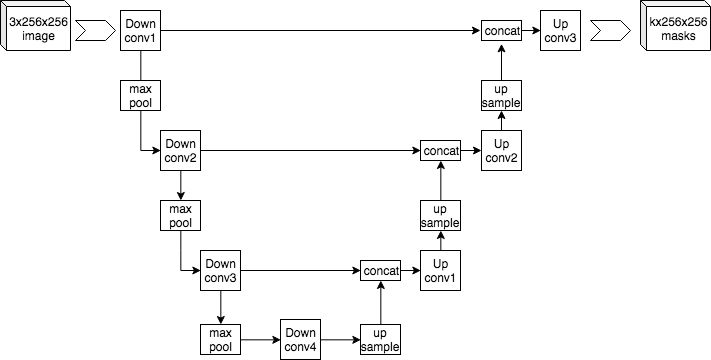
A U-Net with a ResNet18 encoder pre-trained on ImageNet, 14.34M trainable parameters. The encoder keeps the stem and the four residual stages, and feeds feature maps with 64, 128, 256 and 512 channels to the decoder through skip connections. The first convolution is adapted from RGB to one grayscale channel by combining the pre-trained weights, and the decoder ends with a convolution giving one foreground logit per pixel.
The loss is a 50/50 mix of binary cross-entropy and soft Dice. BCE gives per-pixel supervision, Dice looks at overlap and is insensitive to the imbalance:
Training uses AdamW (learning rate , cosine decay, at most 20 epochs) with flips, 90 degree rotations, brightness and contrast jitter and Gaussian noise.
Memory
The project had a resource budget: roughly 5 GB of GPU memory for training and 4 GB for inference (optional thresholds, but I treated them as hard limits). Training ran on a Google Colab instance with an NVIDIA H100, so the limit came from the rules, not from the card.
Resolution mattered most for quality: filaments are thin, and shrinking an image to erases many of them. But a full frame is expensive, and the full-frame variants I tried peaked above 9 GB in training.
What worked was training on random crops of the native image, and at inference covering the frame with four overlapping tiles, blending their probability maps before thresholding. On top of that: gradient accumulation (two crops with batch size 1 for an effective batch of 2), gradient checkpointing and bfloat16 mixed precision. The final model peaks at 3.04 GB in training and 2.53 GB at inference.
Images and rasterised polygon masks are decoded once into memory-mapped uint8 files, so epochs don't repeat JPEG decoding.
Experiments
I ran 22 configurations. These are the ones that changed a decision:
| Exp. | What changed | Dice | PQ |
|---|---|---|---|
| 1 | U-Net from scratch, | 0.6415 | n/a |
| 2 | pre-trained ResNet18 encoder | 0.6552 | 0.2505 |
| 3 | Tversky + clDice loss, | 0.4937 | 0.0618 |
| 5 | input | 0.6665 | 0.4022 |
| 8 | full image at | 0.6678 | 0.4264 |
| 13 | native image, crops | 0.6762 | 0.3591 |
| 15m | full , weighted BCE, memory controls | 0.6650 | 0.4153 |
The first three used a plain 0.5 threshold. The others were scored at native resolution with output settings tuned on validation, so read the table as a trail of evidence, not a strict leaderboard.
- Transfer learning helped. A pre-trained ResNet18 beat the from-scratch encoder, even on grayscale solar images.
- Specialised losses didn't. I assumed fragmentation was a loss problem and tried Tversky and clDice (a topology-aware loss for thin structures). Both metrics collapsed. Fragmentation turned out to be mostly a resolution problem: BCE + Dice with more pixels beat any specialised loss.
- Memory constrained the choice. Run 15 (weighted BCE on a resized frame) had the best PQ among the lighter models, 0.4198, but needed 5.20 GB in training, over budget. 15m is the same idea with accumulation, checkpointing and mixed precision: 2.63 GB peak and 0.4153 PQ.
- Bigger models didn't pay off. ResNet34 used more memory with no Dice gain. Full-resolution U-Nets and YOLOv8 segmentation models raised PQ a little, but YOLOv8x needed 38.74 GB of training memory and still lost on Dice.
Dice or PQ
The network outputs a probability per pixel. Turning it into a mask means choosing a threshold, an optional morphological closing, a minimum component size and an optional confidence gate. I searched these jointly on validation at native resolution.
The best setting depends on the metric. A more selective output removes small spurious components, which helps PQ, but also drops real filament pixels, which hurts Dice. Experiment 13 (threshold 0.30, minimum component size 128 pixels) gives the best Mean Dice, 0.6762, with a PQ of 0.3591. Experiment 15m gets a better PQ (0.4153) and gives up 0.0112 Dice.
Mean Dice was the primary metric, so I delivered experiment 13 and kept 15m as the second candidate (its PQ-oriented submission scored 0.35 on the public leaderboard). Dice and PQ are always reported for the same frozen configuration, never the best of each from different setups.
Among the projects submitted for the exam session I took part in, mine ranked first, and the project got a band A grade.
Where it fails
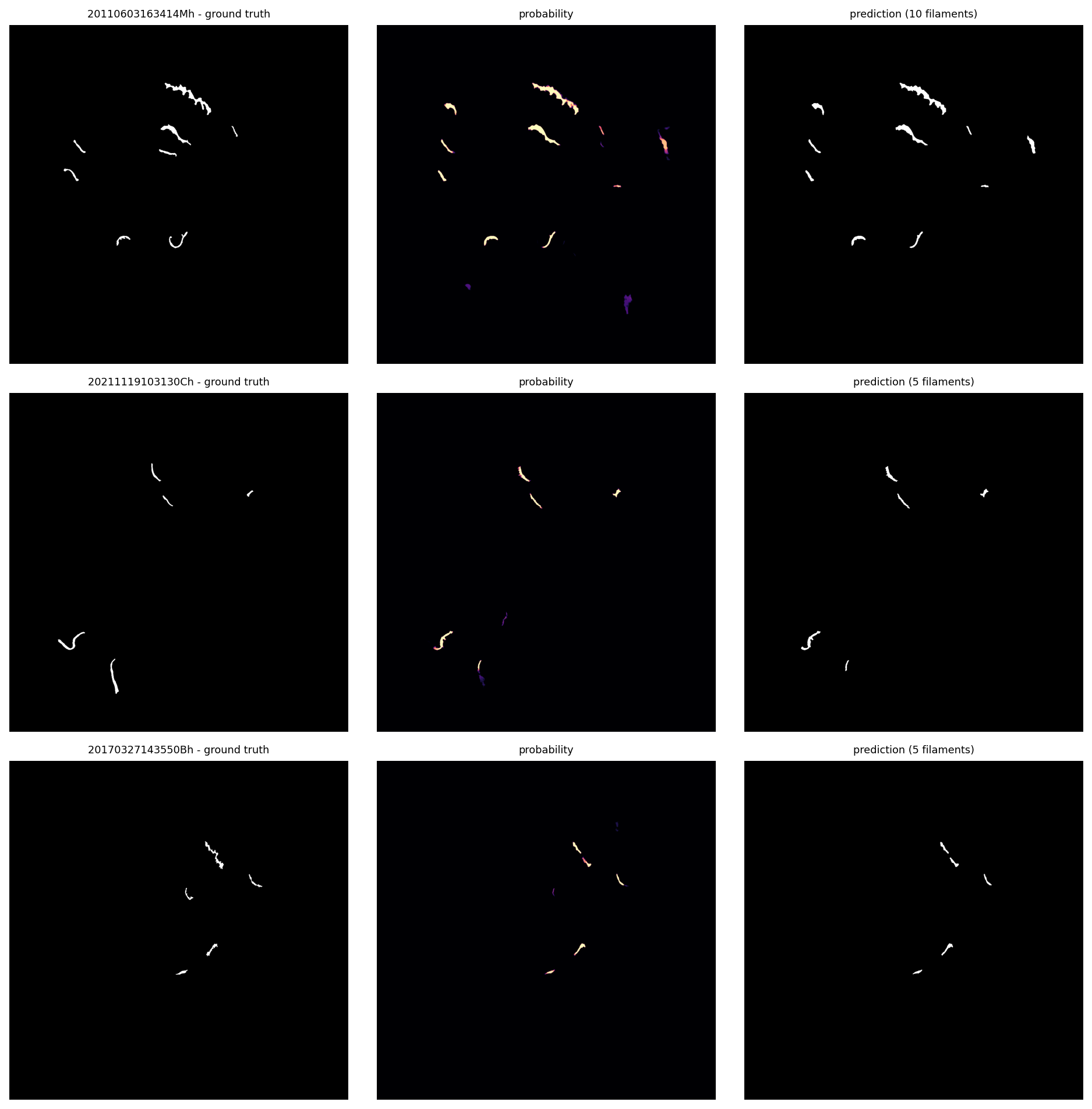
On validation the delivered model gets 733 matched instances, 845 false positives and 411 false negatives. SQ is 0.667 but RQ is only 0.539, so recognition errors cost more PQ than imprecise boundaries.
Size is the clearest weakness. Recall is 0.44 for filaments under 500 pixels, 0.65 between 500 and 1000, and around 0.7 for larger ones. About half the false positives (418 of 845) touch no annotated pixel, so some may be real filaments nobody labelled.
Caveats and next steps
Several experiments changed more than one thing at once (the first transfer learning run changed the learning rate too), so not every gain maps to a single cause, and small differences between runs shouldn't be over-read.
With more time I'd work on the small filaments: recall on tiny, faint structures is where most of the remaining score is.